Backtests vs Reality: DSR Explained

Editorial Note: While we adhere to strict Editorial Integrity, this post may contain references to products from our partners. Here's an explanation for How We Make Money. None of the data and information on this webpage constitutes investment advice according to our Disclaimer.

Backtests often fail to match live trading because they suffer from overfitting and unrealistic assumptions about return distributions. The Deflated Sharpe Ratio (DSR) corrects for both non-normal returns and multiple backtests, giving traders a more realistic measure of whether performance is likely to repeat.

There has been a common theme with my articles so far, and I am going to extend this theme for a few more articles. My goal is to help you gain insights that most traders are missing and that are causing them lots of frustration and, worse, the loss of money.

The idea is to properly understand the risks before committing to a strategy. It is better to experience short-term pain and long-term modest gains versus short-term gain and long-term pain. Yes, you will be frustrated, as it will feel like most of the strategies that you want to trade are not as profitable as your initial backtests might suggest.

I don’t know about you, but I would rather know the ugly truth upfront than fall for an illusion that makes me feel excited and hopeful, only to eventually experience inevitable financial loss and disappointment.

Towards the end of the year, I will be releasing software that is built on the principles I am sharing in these articles. The software will give you the full power of the models introduced and help provide the first backtesting framework that combats the pitfalls that all the traditional backtest software applications enable.

I want to share a little secret. Almost all the professional system developers I have come across, including ones that I have paid subscriptions for, fail to understand the mistakes they are making. It is quite incredible how the human condition is wired to ignore such obvious biases simply because the temptation to feel good right now overwhelms the rational thinking part of the brain. As Daniel Kahneman calls “System 2” in his bestseller, Thinking Fast and Slow.

The academic literature suggests that actual trading results are on average between 35% and 70% worse than the backtest results. Our goal is to align more accurately future live test results with backtest results.

Introducing DSR (Deflated Sharpe Ratio)

There are several challenges to backtesting. In this article we are going to focus on DSR and how it helps combat a couple of typical backtesting pitfalls most experienced and rookie system developers fall for.

The first issue one needs to overcome is that the typical Sharpe Ratio, which is the gold standard for measuring risk-adjusted performance, assumes that returns are normally distributed. We will address this by using some sophisticated techniques to adequately calculate the probability of producing the expected returns the backtest suggests.

The second issue we will address is penalising profitable backtest “cherry-picking”. The industry term refers to it as “curve fitting”. It is when you continuously tweak parameters, for example, different moving average lookback windows, start dates, symbols universe, or a variety of other modifications to find the best backtest. Picture 19 backtest variations with average or below-average results and 1 decent result. The natural tendency is to choose the 1 good result and think you have found the holy grail. We will apply a penalty factor to help us adequately anticipate the probability of this 1 out of 20 good backtests repeating the past.

Non-normal distributions

Let us first discuss what the practical issue is with using a model such as the Sharpe Ratio that assumes normal distribution (it doesn’t really but read on as it will explain where it “slips in”) with the reality of a distribution that is not normal, i.e., it displays skewness and kurtosis.

Skewness measures the asymmetry of returns.
- A positively skewed strategy might deliver frequent small losses and the occasional big win (think of buying lottery tickets or holding long volatility).
- A negatively skewed strategy produces frequent small wins but rare, devastating losses (classic examples: selling options, martingale systems).
Kurtosis measures the “fatness” of the tails.
- A distribution with high kurtosis has a much higher probability of extreme outcomes compared to the normal bell curve.
- This means that rare events (like flash crashes or black swans) happen far more often than the Sharpe-based math would lead you to believe.

Together, skewness and kurtosis explain why many strategies that look smooth on a backtest are ticking time bombs in live trading.

The whole discussion on non-normality and normality is actually more subtle than you might expect. If you are looking for where in the Sharpe Ratio formulae is the normal distribution assumption, you won’t find it. It only shows up in the interpretation of the Sharpe Ratio.

The Raw Sharpe Formula

The Raw Sharpe Formula

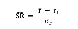
Or in plain English:

Sharpe Ratio = (mean return – risk-free rate) / standard deviation of returns

Here is a Concrete Example when looking at Interpretation of the Sharpe Ratio.

Under normal returns:
A Sharpe of 1 means “expected excess return is 1 standard deviation above zero → probability of a negative excess return ~16%.”

Under non-normal returns:
That mapping breaks down. If returns are negatively skewed with fat tails, the chance of a catastrophic loss is much higher than 16%, even with Sharpe = 1.

This is an illustration of the different return distributions being calibrated for.

Normal vs Skewed vs Fat-Tailored Distributions

We need to now cover a little bit of theory and background, as this is not a trivial subject. The complexity is largely under the hood, and I am going to try and keep it there.

DSR is the creation of 2 of the finest quantitative academics who are themselves practitioners. Bailey and Lopez de Prado. You can read their paper for more details.

PSR

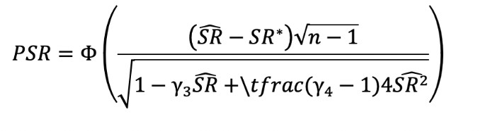
What each symbol means:

SR^: observed Sharpe ratio.
SR*: benchmark Sharpe (often 0).
n: number of return observations.
γ₃: skewness of returns.
γ₄: kurtosis of returns.
Φ: cumulative distribution function (CDF) of the standard normal distribution.

I have a long history with the PSR formulae which is the first step to calculating DSR. It formed the basis of a proprietary scoring algorithm I sold in 2015 called The RAPA Score™️. It is extremely complicated mathematics, I would recommend just working with the concepts for now and avoid trying to understand the math if you are not at a math graduate level.

Deflating the Sharpe Ratio (DSR)

Now that we have introduced PSR, which corrects for non-normal return distributions, we can move to the Deflated Sharpe Ratio (DSR). The DSR takes the probability-adjusted Sharpe (PSR) and adds another crucial correction: it accounts for the fact that you may have run dozens, or even hundreds, of backtests before selecting “the winner.”

This is often referred to as the multiple testing problem. The more you try, the higher the chance that one of those trials will look statistically significant purely by luck. Without correcting for this, you are essentially fooling yourself – you haven’t discovered skill, you’ve discovered randomness.

DSR “deflates” the reported Sharpe by penalizing it for the effective number of trials you performed. In practice, that means a strategy with a Sharpe of 1.0 discovered after 100 different parameter tweaks will end up with a much lower DSR than a strategy with a Sharpe of 0.6 found with minimal tweaking.

Why this matters

This adjustment is not just academic nit-picking. It’s the difference between a strategy that looks like a money machine on paper but fails miserably in live trading, versus a strategy that delivers smaller, more realistic backtest results but has a fighting chance to survive in real markets.

Here are two concrete illustrations:

Example 1: You test 20 variations of a moving average crossover system. Nineteen of them show no edge; one shows a Sharpe of 1.2.
- Traditional Sharpe interpretation: “Great system!”
- DSR interpretation: “This is likely curve-fitting – probability of real skill is low.”
Example 2: You test 3 variations of a breakout strategy. Two show modest results, and one shows a Sharpe of 0.65.
- Traditional Sharpe: “Not very exciting.”
- DSR interpretation: “This may be a robust edge – fewer trials, more consistent behaviour, higher chance of repeatability.”

The chart below shows you visually how the red curve fitted strategy gets adjusted by the PSR and DSR elements of the Bailey and Lopez de Prado contribution to the quantitative community. The effect on a more robust strategy in green is less as you would expect.

Sharpe vs PSR vs DSR

The payoff

By incorporating DSR, you can finally bridge the frustrating gap between glowing backtests and disappointing live trading. Instead of being seduced by the single best run, you can evaluate strategies by their research integrity:

Did they survive tests across time periods and universes?
Did they hold up under parameter jittering?
Did they maintain significance once corrected for multiple trials?

In other words, DSR is a tool to tell you the ugly truth before the market does. And in trading, truth – however painful in the short run – is what keeps you in the game long enough to see real success.

DSR is the first practical step toward holding ourselves accountable

As someone who has spent decades in both research and trading, I’ve seen how seductive a “perfect” backtest can be. The danger lies in believing that a high Sharpe Ratio equates to robustness without questioning how it was achieved. In my experience, most of the strategies that collapse in live trading look amazing in hindsight – because they’ve been heavily optimized. The Deflated Sharpe Ratio is the first practical step toward holding ourselves accountable. It forces us to ask: Did this edge emerge from skill, or from running 100 variations until something looked good? By penalizing curve-fitting and adjusting for non-normal returns, DSR helps filter out illusions of performance. My advice: embrace the discomfort of lower – but more realistic – expectations. The strategies that look modest in backtests but survive the deflation test are the ones most likely to deliver sustainable results in live markets. That mindset shift alone can save years of frustration and significant capital.

Conclusion

The Sharpe Ratio has long been the industry’s gold standard, but its blind spots explain much of the gap between backtests and live trading. By first correcting for skewness and kurtosis with PSR, and then deflating for multiple trials with DSR, traders gain a truer picture of whether a strategy has real merit. In the end, it is better to accept the uncomfortable truth now than to let the markets deliver it later.

FAQs

Why do backtests often fail in live trading?

Because backtests suffer from overfitting, unrealistic assumptions about returns, and the absence of real-world factors like slippage and liquidity.

What is the Deflated Sharpe Ratio?

The DSR is a statistical adjustment to the Sharpe Ratio that corrects for non-normal returns and the multiple testing problem, making results more reliable.

How does curve-fitting affect backtests?

Curve-fitting means tailoring a strategy too closely to historical data, which creates results that look good in the past but are unlikely to repeat in the future.

Is a high Sharpe Ratio always good?

Not necessarily. A high Sharpe may reflect overfitting or exposure to hidden tail risk. Without adjustments like PSR and DSR, it can be misleading.

How can traders make backtests more realistic?

Use robust methods like PSR and DSR, test across different time periods and universes, and penalize strategies that only work after heavy parameter tweaking.

Did you like the article?

Editors' Top Picks and Insights

52 minutes ago Eugene Komchuk

Five years with Bitcoin: How El Salvador changed after legalizing BTC

#Nayib Bukele #Bitcoin

1 day ago Anastasiia Chabaniuk

Crypto on the court: How NBA Finals became a showcase for Ledger

#Ledger #Crypto

1 day ago Johnathan Maverick

How to build wealth from scratch in 3 practical steps

#Finance #NVDA #Apple

2 days ago Eugene Komchuk

Kospi Index crash: Why South Korean market fell alongside AI stocks

#Finance #Stocks #Stock indexes

2 days ago Mira Kyivska

Bitcoin or Ferrari: Which investment is better?

#Crypto #Bitcoin

3 days ago Mira Kyivska

Strategy sells Bitcoin: Small sale tests market confidence

#Michael Saylor #Crypto #Bitcoin #Strategy

All news

Team that worked on the article

Michael has decades of experience as a professional trader, hedge fund manager and incubator of emerging traders. He has built a number of trading analytic platforms with 3 successful exits and has served as the CEO of a regulated CFD broker and as a director of a public company in his late 20’s.

Learn about our editorial policies

Dan Blystone began his trading career in 1998 as an arbitrage clerk on the floor of the Chicago Mercantile Exchange (CME). He later traded bond and Eurex futures at proprietary firms such as Altea Trading, gaining valuable experience in high-frequency trading and risk management.

Chinmay Soni is a financial analyst with more than 5 years of experience in working with stocks, Forex, derivatives, and other assets. As a founder of a boutique research firm and an active researcher, he covers various industries and fields, providing insights backed by statistical data.

Black swans

Black swans are a term that was introduced by Nassim Taleb, denoting global unpredictable events that can radically change the situation.

Backtesting

Backtesting is the process of testing a trading strategy on historical data. It allows you to evaluate the strategy's performance in the past and identify its potential risks and benefits.

Volatility

Volatility refers to the degree of variation or fluctuation in the price or value of a financial asset, such as stocks, bonds, or cryptocurrencies, over a period of time. Higher volatility indicates that an asset's price is experiencing more significant and rapid price swings, while lower volatility suggests relatively stable and gradual price movements.

Investor

An investor is an individual, who invests money in an asset with the expectation that its value would appreciate in the future. The asset can be anything, including a bond, debenture, mutual fund, equity, gold, silver, exchange-traded funds (ETFs), and real-estate property.

Deviation

The deviation is a statistical measure of how much a set of data varies from the mean or average value. In forex trading, this measure is often calculated using standard deviation that helps traders in assessing the degree of variability or volatility in currency price movements.

Top 5 companies for you